Bioinformatics Portfolio
My coursework from BIMM 143. Showcasing genomic analysis techniques, introductory machine learning, and protein folding and structure prediction.
Class 14: RNASeq Mini-Project
Aadhya Tripathi (PID: A17878439
Background
The data for today’s mini-project comes from a knock-down study of an important HOX gene.
Data Import
Import counts data and metadata:
countData <- read.csv("GSE37704_featurecounts.csv", row.names = 1)
colData <- read.csv("GSE37704_metadata.csv", row.names = 1)
Quick look at the imports:
head(countData)
                length SRR493366 SRR493367 SRR493368 SRR493369 SRR493370
ENSG00000186092    918         0         0         0         0         0
ENSG00000279928    718         0         0         0         0         0
ENSG00000279457   1982        23        28        29        29        28
ENSG00000278566    939         0         0         0         0         0
ENSG00000273547    939         0         0         0         0         0
ENSG00000187634   3214       124       123       205       207       212
                SRR493371
ENSG00000186092         0
ENSG00000279928         0
ENSG00000279457        46
ENSG00000278566         0
ENSG00000273547         0
ENSG00000187634       258
head(colData)
              condition
SRR493366 control_sirna
SRR493367 control_sirna
SRR493368 control_sirna
SRR493369      hoxa1_kd
SRR493370      hoxa1_kd
SRR493371      hoxa1_kd
Data Cleanup
Remove length column in countData:
countData <- as.matrix(countData[,-1])
Check if the countData columns and colData rows match:
colnames(countData) == rownames(colData)
[1] TRUE TRUE TRUE TRUE TRUE TRUE
Remove genes with no expression:
countData = countData[rowSums(countData) > 0, ]
head(countData)
                SRR493366 SRR493367 SRR493368 SRR493369 SRR493370 SRR493371
ENSG00000279457        23        28        29        29        28        46
ENSG00000187634       124       123       205       207       212       258
ENSG00000188976      1637      1831      2383      1226      1326      1504
ENSG00000187961       120       153       180       236       255       357
ENSG00000187583        24        48        65        44        48        64
ENSG00000187642         4         9        16        14        16        16
DESeq Analysis
Setting up the DESeq object
library(DESeq2)
Build the required DESeqDataSet object for DESeq analysis:
dds <- DESeqDataSetFromMatrix(countData = countData,
                             colData = colData,
                             design = ~condition)
Warning in DESeqDataSet(se, design = design, ignoreRank): some variables in
design formula are characters, converting to factors
Running DESeq
Run DESeq on dds:
dds <- DESeq(dds)
estimating size factors

estimating dispersions

gene-wise dispersion estimates

mean-dispersion relationship

final dispersion estimates

fitting model and testing
Getting Results
Save results from running DESeq:
res <- results(dds)
head(res)
log2 fold change (MLE): condition hoxa1 kd vs control sirna
Wald test p-value: condition hoxa1 kd vs control sirna
DataFrame with 6 rows and 6 columns
                 baseMean log2FoldChange     lfcSE       stat      pvalue
                <numeric>      <numeric> <numeric>  <numeric>   <numeric>
ENSG00000279457   29.9136      0.1792571 0.3248216   0.551863 5.81042e-01
ENSG00000187634  183.2296      0.4264571 0.1402658   3.040350 2.36304e-03
ENSG00000188976 1651.1881     -0.6927205 0.0548465 -12.630158 1.43990e-36
ENSG00000187961  209.6379      0.7297556 0.1318599   5.534326 3.12428e-08
ENSG00000187583   47.2551      0.0405765 0.2718928   0.149237 8.81366e-01
ENSG00000187642   11.9798      0.5428105 0.5215598   1.040744 2.97994e-01
                       padj
                  <numeric>
ENSG00000279457 6.86555e-01
ENSG00000187634 5.15718e-03
ENSG00000188976 1.76549e-35
ENSG00000187961 1.13413e-07
ENSG00000187583 9.19031e-01
ENSG00000187642 4.03379e-01
Visualization: Volcano Plot
library(ggplot2)
Create basic volcano plot of Log2 Fold Change vs -Log of Adjusted P-value in DESeq results:
ggplot(res) +
      aes(x=log2FoldChange,
          y=-log(padj)) +
      geom_point()
Warning: Removed 1237 rows containing missing values or values outside the scale range
(`geom_point()`).

Improve the plot with color and lines to highlight significant changes.
my_cols <- rep("gray", nrow(res))
my_cols[abs(res$log2FoldChange) > 2 ] <- "blue"
my_cols[res$padj>=0.01] <- "gray"
ggplot(res) +
      aes(x=log2FoldChange,
          y=-log(padj)) +
      geom_point(col=my_cols) +
      geom_vline(xintercept = c(-2,+2), col="red") +
      geom_hline(yintercept = -log(0.01), col="red") +
      labs(x = "Log2(Fold Change)",
           y = "-Log(Adjusted P-value)",
           title = "Volcano plot of Log2(Fold Change) vs -Log(Adjusted P-value)")
Warning: Removed 1237 rows containing missing values or values outside the scale range
(`geom_point()`).

Save the results of DESeq analysis to a csv file:
write.csv(res, file="results.csv")
Add Annotation
library("AnnotationDbi")
library("org.Hs.eg.db")
List of all available key types for mapping:
columns(org.Hs.eg.db)
 [1] "ACCNUM"       "ALIAS"        "ENSEMBL"      "ENSEMBLPROT"  "ENSEMBLTRANS"
 [6] "ENTREZID"     "ENZYME"       "EVIDENCE"     "EVIDENCEALL"  "GENENAME"
[11] "GENETYPE"     "GO"           "GOALL"        "IPI"          "MAP"
[16] "OMIM"         "ONTOLOGY"     "ONTOLOGYALL"  "PATH"         "PFAM"
[21] "PMID"         "PROSITE"      "REFSEQ"       "SYMBOL"       "UCSCKG"
[26] "UNIPROT"
Add columns to res to save information on the SYMBOL, ENTREZ ID, and
gene names.
res$symbol = mapIds(org.Hs.eg.db,
                    keys=rownames(res),
                    keytype="ENSEMBL",
                    column="SYMBOL",
                    multiVals="first")
'select()' returned 1:many mapping between keys and columns
res$entrez = mapIds(org.Hs.eg.db,
                    keys=row.names(res),
                    keytype="ENSEMBL",
                    column="ENTREZID",
                    multiVals="first")
'select()' returned 1:many mapping between keys and columns
res$name =   mapIds(org.Hs.eg.db,
                    keys=row.names(res),
                    keytype="ENSEMBL",
                    column="GENENAME",
                    multiVals="first")
'select()' returned 1:many mapping between keys and columns
Quick look at res with the new columns:
head(res)
log2 fold change (MLE): condition hoxa1 kd vs control sirna
Wald test p-value: condition hoxa1 kd vs control sirna
DataFrame with 6 rows and 9 columns
                 baseMean log2FoldChange     lfcSE       stat      pvalue
                <numeric>      <numeric> <numeric>  <numeric>   <numeric>
ENSG00000279457   29.9136      0.1792571 0.3248216   0.551863 5.81042e-01
ENSG00000187634  183.2296      0.4264571 0.1402658   3.040350 2.36304e-03
ENSG00000188976 1651.1881     -0.6927205 0.0548465 -12.630158 1.43990e-36
ENSG00000187961  209.6379      0.7297556 0.1318599   5.534326 3.12428e-08
ENSG00000187583   47.2551      0.0405765 0.2718928   0.149237 8.81366e-01
ENSG00000187642   11.9798      0.5428105 0.5215598   1.040744 2.97994e-01
                       padj      symbol      entrez                   name
                  <numeric> <character> <character>            <character>
ENSG00000279457 6.86555e-01          NA          NA                     NA
ENSG00000187634 5.15718e-03      SAMD11      148398 sterile alpha motif ..
ENSG00000188976 1.76549e-35       NOC2L       26155 NOC2 like nucleolar ..
ENSG00000187961 1.13413e-07      KLHL17      339451 kelch like family me..
ENSG00000187583 9.19031e-01     PLEKHN1       84069 pleckstrin homology ..
ENSG00000187642 4.03379e-01       PERM1       84808 PPARGC1 and ESRR ind..
Save the annotated results to a csv file:
write.csv(res, file="results_annotated.csv")
Pathway Analysis
library(pathview)
##############################################################################
Pathview is an open source software package distributed under GNU General
Public License version 3 (GPLv3). Details of GPLv3 is available at
http://www.gnu.org/licenses/gpl-3.0.html. Particullary, users are required to
formally cite the original Pathview paper (not just mention it) in publications
or products. For details, do citation("pathview") within R.

The pathview downloads and uses KEGG data. Non-academic uses may require a KEGG
license agreement (details at http://www.kegg.jp/kegg/legal.html).
##############################################################################
library(gage)
library(gageData)
KEGG
data(kegg.sets.hs)
data(sigmet.idx.hs)

kegg.sets.hs = kegg.sets.hs[sigmet.idx.hs]
Create foldchanges vector, which is needed for gage()
foldchanges <- res$log2FoldChange
names(foldchanges) <- res$entrez
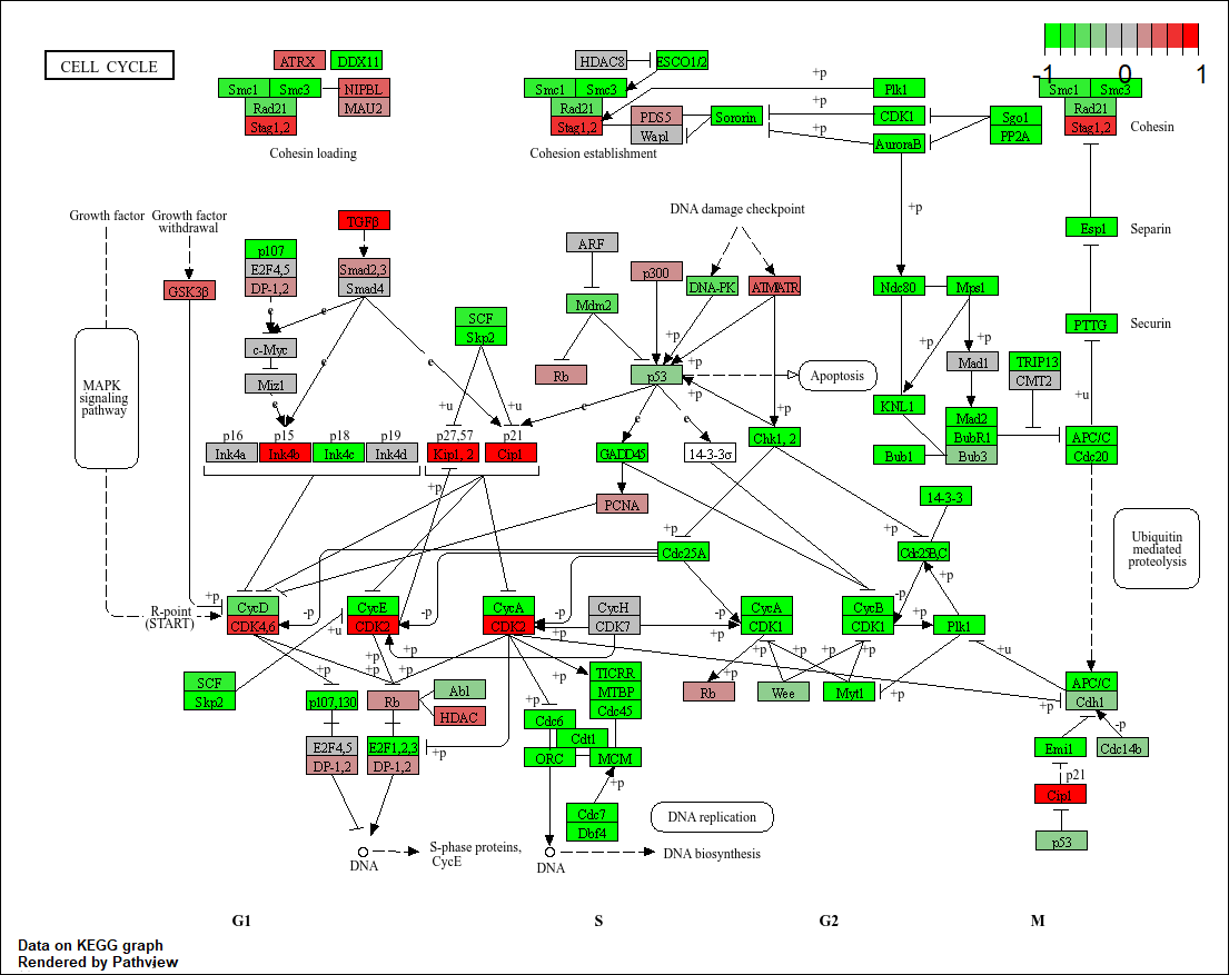
keggres <- gage(foldchanges, gsets=kegg.sets.hs)
pathview(gene.data=foldchanges, pathway.id="hsa04110")
'select()' returned 1:1 mapping between keys and columns

Info: Working in directory C:/Users/extra/Documents/school/BIMM 143/bimm143_github/class14

Info: Writing image file hsa04110.pathview.png
GO
data(go.sets.hs)
data(go.subs.hs)
# Focus on Biological Process subset of GO
gobpsets = go.sets.hs[go.subs.hs$BP]

gobpres = gage(foldchanges, gsets=gobpsets)
head(gobpres$less)
                                            p.geomean stat.mean        p.val
GO:0048285 organelle fission             1.536227e-15 -8.063910 1.536227e-15
GO:0000280 nuclear division              4.286961e-15 -7.939217 4.286961e-15
GO:0007067 mitosis                       4.286961e-15 -7.939217 4.286961e-15
GO:0000087 M phase of mitotic cell cycle 1.169934e-14 -7.797496 1.169934e-14
GO:0007059 chromosome segregation        2.028624e-11 -6.878340 2.028624e-11
GO:0000236 mitotic prometaphase          1.729553e-10 -6.695966 1.729553e-10
                                                q.val set.size         exp1
GO:0048285 organelle fission             5.841698e-12      376 1.536227e-15
GO:0000280 nuclear division              5.841698e-12      352 4.286961e-15
GO:0007067 mitosis                       5.841698e-12      352 4.286961e-15
GO:0000087 M phase of mitotic cell cycle 1.195672e-11      362 1.169934e-14
GO:0007059 chromosome segregation        1.658603e-08      142 2.028624e-11
GO:0000236 mitotic prometaphase          1.178402e-07       84 1.729553e-10
Reactome
sig_genes <- res[res$padj <= 0.05 & !is.na(res$padj), "symbol"]
print(paste("Total number of significant genes:", length(sig_genes)))
[1] "Total number of significant genes: 8147"
write.table(sig_genes, file="significant_genes.txt", row.names=FALSE, col.names=FALSE, quote=FALSE)