Bioinformatics Portfolio
My coursework from BIMM 143. Showcasing genomic analysis techniques, introductory machine learning, and protein folding and structure prediction.
Class 11: AlphaFold
Aadhya Tripathi (PID: A17878439)
- Background
- EBI AlphaFold Database
- Running AlphaFold
- Analysis of Resulting Models
- Predicted Alignment Error for domains
Background
In this hands-on session we will utilize AlphaFold to predict protein structure from sequence (Jumper et al. 2021).
Without the aid of such approaches, it can take years of expensive laboratory work to determine the structure of just one protein. With AlphaFold we can now accurately compute a typical protein structure in as little as ten minutes.
The PDB database (the main repository of experimental structures) only has ~250 thousand structures, as we saw in the last lab. The main protein sequence database has >200 million sequences! Only 0.125% of known sequences have a known structure. This is called the “structure knowledge gap”.
250000 / 200000000
[1] 0.00125
- Structures are much harder to determine than sequences.
- They are expensive (costing $1M on average).
- They take an average of 3-5 years to solve.
EBI AlphaFold Database
The EBI has a database of pre-computed AlphaFold (AF) models called AFDB. This is growing all the time and can be useful to check before running AF ourselves.
Running AlphaFold
We can download and run locally but we need a GPU. Or we can use “cloud” computing to run this on someone else’s computer!
We will use ColabFold https://github.com/sokrypton/ColabFold
We previously found there was no AFDB entry for our HIV sequence.
>HIV-Pr-Dimer
PQITLWQRPLVTIKIGGQLKEALLDTGADDTVLEEMSLPGRWKPKMIGGIGGFIKVRQYDQILIEICGHKAIGTVLVGPTPVNIIGRNLLTQIGCTLNF:PQITLWQRPLVTIKIGGQLKEALLDTGADDTVLEEMSLPGRWKPKMIGGIGGFIKVRQYDQILIEICGHKAIGTVLVGPTPVNIIGRNLLTQIGCTLNF
Here we will use AlphaFold2_mmseqs2.
![]()
Analysis of Resulting Models
Save AlphaFold2 prediction results and import
results_dir <- "HIV_23119/"
pdb_files <- list.files(path=results_dir,
                        pattern="*.pdb",
                        full.names = TRUE)

# Print our PDB file names
basename(pdb_files)
[1] "HIV_23119_unrelaxed_rank_001_alphafold2_multimer_v3_model_4_seed_000.pdb"
[2] "HIV_23119_unrelaxed_rank_002_alphafold2_multimer_v3_model_1_seed_000.pdb"
[3] "HIV_23119_unrelaxed_rank_003_alphafold2_multimer_v3_model_5_seed_000.pdb"
[4] "HIV_23119_unrelaxed_rank_004_alphafold2_multimer_v3_model_2_seed_000.pdb"
[5] "HIV_23119_unrelaxed_rank_005_alphafold2_multimer_v3_model_3_seed_000.pdb"
Load bio3d and save top 5 ranked models
library(bio3d)
pdbs <- pdbaln(pdb_files, fit=TRUE, exefile="msa")
Reading PDB files:
HIV_23119/HIV_23119_unrelaxed_rank_001_alphafold2_multimer_v3_model_4_seed_000.pdb
HIV_23119/HIV_23119_unrelaxed_rank_002_alphafold2_multimer_v3_model_1_seed_000.pdb
HIV_23119/HIV_23119_unrelaxed_rank_003_alphafold2_multimer_v3_model_5_seed_000.pdb
HIV_23119/HIV_23119_unrelaxed_rank_004_alphafold2_multimer_v3_model_2_seed_000.pdb
HIV_23119/HIV_23119_unrelaxed_rank_005_alphafold2_multimer_v3_model_3_seed_000.pdb
.....

Extracting sequences

pdb/seq: 1   name: HIV_23119/HIV_23119_unrelaxed_rank_001_alphafold2_multimer_v3_model_4_seed_000.pdb
pdb/seq: 2   name: HIV_23119/HIV_23119_unrelaxed_rank_002_alphafold2_multimer_v3_model_1_seed_000.pdb
pdb/seq: 3   name: HIV_23119/HIV_23119_unrelaxed_rank_003_alphafold2_multimer_v3_model_5_seed_000.pdb
pdb/seq: 4   name: HIV_23119/HIV_23119_unrelaxed_rank_004_alphafold2_multimer_v3_model_2_seed_000.pdb
pdb/seq: 5   name: HIV_23119/HIV_23119_unrelaxed_rank_005_alphafold2_multimer_v3_model_3_seed_000.pdb
pdbs
                               1        .         .         .         .         50
[Truncated_Name:1]HIV_23119_   PQITLWQRPLVTIKIGGQLKEALLDTGADDTVLEEMSLPGRWKPKMIGGI
[Truncated_Name:2]HIV_23119_   PQITLWQRPLVTIKIGGQLKEALLDTGADDTVLEEMSLPGRWKPKMIGGI
[Truncated_Name:3]HIV_23119_   PQITLWQRPLVTIKIGGQLKEALLDTGADDTVLEEMSLPGRWKPKMIGGI
[Truncated_Name:4]HIV_23119_   PQITLWQRPLVTIKIGGQLKEALLDTGADDTVLEEMSLPGRWKPKMIGGI
[Truncated_Name:5]HIV_23119_   PQITLWQRPLVTIKIGGQLKEALLDTGADDTVLEEMSLPGRWKPKMIGGI
                               **************************************************
                               1        .         .         .         .         50

                              51        .         .         .         .         100
[Truncated_Name:1]HIV_23119_   GGFIKVRQYDQILIEICGHKAIGTVLVGPTPVNIIGRNLLTQIGCTLNFP
[Truncated_Name:2]HIV_23119_   GGFIKVRQYDQILIEICGHKAIGTVLVGPTPVNIIGRNLLTQIGCTLNFP
[Truncated_Name:3]HIV_23119_   GGFIKVRQYDQILIEICGHKAIGTVLVGPTPVNIIGRNLLTQIGCTLNFP
[Truncated_Name:4]HIV_23119_   GGFIKVRQYDQILIEICGHKAIGTVLVGPTPVNIIGRNLLTQIGCTLNFP
[Truncated_Name:5]HIV_23119_   GGFIKVRQYDQILIEICGHKAIGTVLVGPTPVNIIGRNLLTQIGCTLNFP
                               **************************************************
                              51        .         .         .         .         100

                             101        .         .         .         .         150
[Truncated_Name:1]HIV_23119_   QITLWQRPLVTIKIGGQLKEALLDTGADDTVLEEMSLPGRWKPKMIGGIG
[Truncated_Name:2]HIV_23119_   QITLWQRPLVTIKIGGQLKEALLDTGADDTVLEEMSLPGRWKPKMIGGIG
[Truncated_Name:3]HIV_23119_   QITLWQRPLVTIKIGGQLKEALLDTGADDTVLEEMSLPGRWKPKMIGGIG
[Truncated_Name:4]HIV_23119_   QITLWQRPLVTIKIGGQLKEALLDTGADDTVLEEMSLPGRWKPKMIGGIG
[Truncated_Name:5]HIV_23119_   QITLWQRPLVTIKIGGQLKEALLDTGADDTVLEEMSLPGRWKPKMIGGIG
                               **************************************************
                             101        .         .         .         .         150

                             151        .         .         .         .       198
[Truncated_Name:1]HIV_23119_   GFIKVRQYDQILIEICGHKAIGTVLVGPTPVNIIGRNLLTQIGCTLNF
[Truncated_Name:2]HIV_23119_   GFIKVRQYDQILIEICGHKAIGTVLVGPTPVNIIGRNLLTQIGCTLNF
[Truncated_Name:3]HIV_23119_   GFIKVRQYDQILIEICGHKAIGTVLVGPTPVNIIGRNLLTQIGCTLNF
[Truncated_Name:4]HIV_23119_   GFIKVRQYDQILIEICGHKAIGTVLVGPTPVNIIGRNLLTQIGCTLNF
[Truncated_Name:5]HIV_23119_   GFIKVRQYDQILIEICGHKAIGTVLVGPTPVNIIGRNLLTQIGCTLNF
                               ************************************************
                             151        .         .         .         .       198

Call:
  pdbaln(files = pdb_files, fit = TRUE, exefile = "msa")

Class:
  pdbs, fasta

Alignment dimensions:
  5 sequence rows; 198 position columns (198 non-gap, 0 gap)

+ attr: xyz, resno, b, chain, id, ali, resid, sse, call
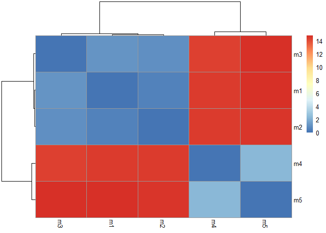
Calculate RMSD between all pairs models:
rd <- rmsd(pdbs, fit=T)
Warning in rmsd(pdbs, fit = T): No indices provided, using the 198 non NA positions
range(rd)
[1] 0.000 14.754
library(pheatmap)
Heatmap of pairs models:
colnames(rd) <- paste0("m",1:5)
rownames(rd) <- paste0("m",1:5)
pheatmap(rd)
# reference PDB structure
pdb <- read.pdb("1hsg")
Note: Accessing on-line PDB file
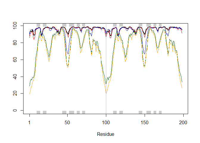
Plot the pLDDT values across all models:
plotb3(pdbs$b[1,], typ="l", lwd=2, sse=pdb)
points(pdbs$b[2,], typ="l", col="red")
points(pdbs$b[3,], typ="l", col="blue")
points(pdbs$b[4,], typ="l", col="darkgreen")
points(pdbs$b[5,], typ="l", col="orange")
abline(v=100, col="gray")
Find most consistent “rigid core” common across all the models:
core <- core.find(pdbs)
 core size 197 of 198  vol = 9885.822
 core size 196 of 198  vol = 6896.71
 core size 195 of 198  vol = 1337.847
 core size 194 of 198  vol = 1040.67
 core size 193 of 198  vol = 951.857
 core size 192 of 198  vol = 899.083
 core size 191 of 198  vol = 834.732
 core size 190 of 198  vol = 771.338
 core size 189 of 198  vol = 733.065
 core size 188 of 198  vol = 697.28
 core size 187 of 198  vol = 659.742
 core size 186 of 198  vol = 625.273
 core size 185 of 198  vol = 589.541
 core size 184 of 198  vol = 568.253
 core size 183 of 198  vol = 545.015
 core size 182 of 198  vol = 512.889
 core size 181 of 198  vol = 490.723
 core size 180 of 198  vol = 470.266
 core size 179 of 198  vol = 450.731
 core size 178 of 198  vol = 434.735
 core size 177 of 198  vol = 420.337
 core size 176 of 198  vol = 406.658
 core size 175 of 198  vol = 393.334
 core size 174 of 198  vol = 382.395
 core size 173 of 198  vol = 372.858
 core size 172 of 198  vol = 356.994
 core size 171 of 198  vol = 346.567
 core size 170 of 198  vol = 337.446
 core size 169 of 198  vol = 326.659
 core size 168 of 198  vol = 314.95
 core size 167 of 198  vol = 304.127
 core size 166 of 198  vol = 294.552
 core size 165 of 198  vol = 285.648
 core size 164 of 198  vol = 278.884
 core size 163 of 198  vol = 266.765
 core size 162 of 198  vol = 258.994
 core size 161 of 198  vol = 247.723
 core size 160 of 198  vol = 239.84
 core size 159 of 198  vol = 234.963
 core size 158 of 198  vol = 230.062
 core size 157 of 198  vol = 221.985
 core size 156 of 198  vol = 215.62
 core size 155 of 198  vol = 206.793
 core size 154 of 198  vol = 196.984
 core size 153 of 198  vol = 188.539
 core size 152 of 198  vol = 182.262
 core size 151 of 198  vol = 176.954
 core size 150 of 198  vol = 170.712
 core size 149 of 198  vol = 166.119
 core size 148 of 198  vol = 159.796
 core size 147 of 198  vol = 153.767
 core size 146 of 198  vol = 149.092
 core size 145 of 198  vol = 143.657
 core size 144 of 198  vol = 137.138
 core size 143 of 198  vol = 132.517
 core size 142 of 198  vol = 127.231
 core size 141 of 198  vol = 121.574
 core size 140 of 198  vol = 116.775
 core size 139 of 198  vol = 112.57
 core size 138 of 198  vol = 108.17
 core size 137 of 198  vol = 105.133
 core size 136 of 198  vol = 101.249
 core size 135 of 198  vol = 97.374
 core size 134 of 198  vol = 92.974
 core size 133 of 198  vol = 88.184
 core size 132 of 198  vol = 84.029
 core size 131 of 198  vol = 81.898
 core size 130 of 198  vol = 78.019
 core size 129 of 198  vol = 75.272
 core size 128 of 198  vol = 73.052
 core size 127 of 198  vol = 70.695
 core size 126 of 198  vol = 68.975
 core size 125 of 198  vol = 66.694
 core size 124 of 198  vol = 64.394
 core size 123 of 198  vol = 62.092
 core size 122 of 198  vol = 59.045
 core size 121 of 198  vol = 56.629
 core size 120 of 198  vol = 54.016
 core size 119 of 198  vol = 51.806
 core size 118 of 198  vol = 49.652
 core size 117 of 198  vol = 48.193
 core size 116 of 198  vol = 46.648
 core size 115 of 198  vol = 44.752
 core size 114 of 198  vol = 43.292
 core size 113 of 198  vol = 41.093
 core size 112 of 198  vol = 39.147
 core size 111 of 198  vol = 36.472
 core size 110 of 198  vol = 34.117
 core size 109 of 198  vol = 31.47
 core size 108 of 198  vol = 29.448
 core size 107 of 198  vol = 27.325
 core size 106 of 198  vol = 25.822
 core size 105 of 198  vol = 24.15
 core size 104 of 198  vol = 22.648
 core size 103 of 198  vol = 21.069
 core size 102 of 198  vol = 19.953
 core size 101 of 198  vol = 18.3
 core size 100 of 198  vol = 15.723
 core size 99 of 198  vol = 14.841
 core size 98 of 198  vol = 11.646
 core size 97 of 198  vol = 9.434
 core size 96 of 198  vol = 7.354
 core size 95 of 198  vol = 6.179
 core size 94 of 198  vol = 5.666
 core size 93 of 198  vol = 4.705
 core size 92 of 198  vol = 3.665
 core size 91 of 198  vol = 2.77
 core size 90 of 198  vol = 2.151
 core size 89 of 198  vol = 1.715
 core size 88 of 198  vol = 1.15
 core size 87 of 198  vol = 0.874
 core size 86 of 198  vol = 0.685
 core size 85 of 198  vol = 0.528
 core size 84 of 198  vol = 0.37
 FINISHED: Min vol ( 0.5 ) reached
core.inds <- print(core, vol=0.5)
# 85 positions (cumulative volume <= 0.5 Angstrom^3)
  start end length
1     9  49     41
2    52  95     44
xyz <- pdbfit(pdbs, core.inds, outpath="corefit_structures")
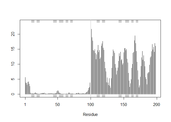
RMSF between positions of the structure:
rf <- rmsf(xyz)

plotb3(rf, sse=pdb)
abline(v=100, col="gray", ylab="RMSF")
Predicted Alignment Error for domains
library(jsonlite)
Access Predicted Aligned Error files:
pae_files <- list.files(path=results_dir,
                        pattern=".*model.*\\.json",
                        full.names = TRUE)
PAE files for Model 1 and 5:
pae1 <- read_json(pae_files[1],simplifyVector = TRUE)
pae5 <- read_json(pae_files[5],simplifyVector = TRUE)

attributes(pae1)
$names
[1] "plddt"   "max_pae" "pae"     "ptm"     "iptm"
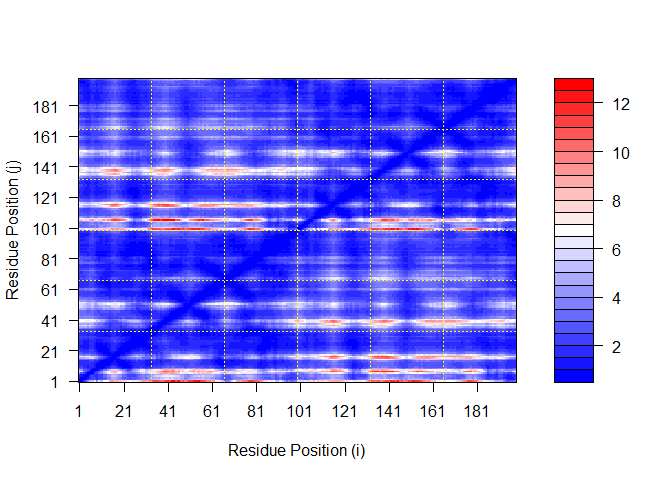
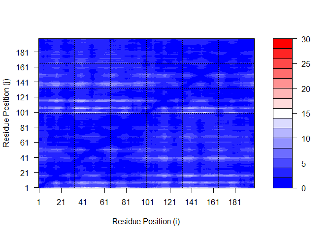
Plot N by N PAE scores for Model 1:
plot.dmat(pae1$pae,
          xlab="Residue Position (i)",
          ylab="Residue Position (j)")
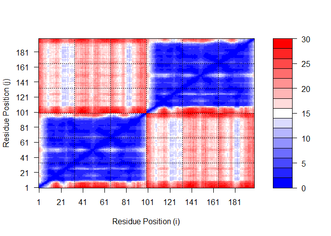
Plot N by N PAE scores for Model 5:
plot.dmat(pae5$pae,
          xlab="Residue Position (i)",
          ylab="Residue Position (j)",
          grid.col = "black",
          zlim=c(0,30))
Plot N by N PAE scores for Model 1 again, using the same data range as the plot for model 5:
plot.dmat(pae1$pae,
          xlab="Residue Position (i)",
          ylab="Residue Position (j)",
          grid.col = "black",
          zlim=c(0,30))
 ## Residue
conservation from alignment file
## Residue
conservation from alignment file
aln_file <- list.files(path=results_dir,
                       pattern=".a3m$",
                        full.names = TRUE)
aln_file
[1] "HIV_23119/HIV_23119.a3m"
aln <- read.fasta(aln_file[1], to.upper = TRUE)
[1] " ** Duplicated sequence id's: 101 **"
[2] " ** Duplicated sequence id's: 101 **"
Number of sequences in alignment
dim(aln$ali)
[1] 5397 132
Score residue conservation in the alignment
sim <- conserv(aln)
plotb3(sim[1:99], sse=trim.pdb(pdb, chain="A"),
       ylab="Conservation Score")
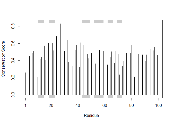
Conserved active sites:
con <- consensus(aln, cutoff = 0.9)
con$seq
  [1] "-" "-" "-" "-" "-" "-" "-" "-" "-" "-" "-" "-" "-" "-" "-" "-" "-" "-"
 [19] "-" "-" "-" "-" "-" "-" "D" "T" "G" "A" "-" "-" "-" "-" "-" "-" "-" "-"
 [37] "-" "-" "-" "-" "-" "-" "-" "-" "-" "-" "-" "-" "-" "-" "-" "-" "-" "-"
 [55] "-" "-" "-" "-" "-" "-" "-" "-" "-" "-" "-" "-" "-" "-" "-" "-" "-" "-"
 [73] "-" "-" "-" "-" "-" "-" "-" "-" "-" "-" "-" "-" "-" "-" "-" "-" "-" "-"
 [91] "-" "-" "-" "-" "-" "-" "-" "-" "-" "-" "-" "-" "-" "-" "-" "-" "-" "-"
[109] "-" "-" "-" "-" "-" "-" "-" "-" "-" "-" "-" "-" "-" "-" "-" "-" "-" "-"
[127] "-" "-" "-" "-" "-" "-"
Save a PDB file with an Occupancy column with conservation scores for visualization.
m1.pdb <- read.pdb(pdb_files[1])
occ <- vec2resno(c(sim[1:99], sim[1:99]), m1.pdb$atom$resno)
write.pdb(m1.pdb, o=occ, file="m1_conserv.pdb")